Linear regression with PyTorch
LBFGS vs Adam
I am looking at using PyTorch for the machine learning component of one the research projects that I am currently working on. It involves regression with relatively small tabular datasets. The data is produced by computer simulations. Though highly nonlinear there is no noise. I am using shallow (1 – 2 hidden layers) neural networks for this purpose. This is an atypical use of PyTorch. I did some prototyping with the simpler neural network library from scikit-learn. While the prototype performs as expected scikit-learn does not have GPU support. Hence PyTorch. One question might be why do I need GPU support for shallow models and small datasets. The answer is that even though the models are shallow I am using a bazillion of them for generalization and uncertainty estimation. The approach can benefit from the parallelization offered by GPUs. Anyways it gave me an excuse to play with PyTorch in ways I have not done before.
For scientific research projects, like the one I am involved in, convergence is important. Second-order optimizers like LBFGS or Levenberg-Marquardt are generally better at convergence than first-order optimizers like SGD or Adam. But only a few handful of machine learning libraries include second-order optimizers. Both scikit-learn and PyTorch provide an LBFGS optimizer. Matlab provides Levenberg-Marquardt among others. 1 There is also a relatively less known neural network library called Pyrenn, which provides Levenberg-Marquardt. As far as I know no other machine learning library provides second-order optimizers for training neural networks. This is because second order optimizers require quadratic storage and cubic computation time for each gradient update. 2 This quickly becomes infeasible for large datasets and deep models, which is what most modern machine learning libraries are used for. For my project this is not an issue.
The LBFGS optimizer that comes with PyTorch lacks certain features, such as mini-batch training, and weak Wolfe line search. Mini-batch training is not very important in my case since the datasets are small. I do not know enough about backtracking line search to know if the lack of it would be important. 3 There are other third-party implementations of the LBFGS optimizer for PyTorch which overcome some of these shortcomings. 4 I wanted to eplore the performance of the builtin LBFGS optimizer, and see if it is adequate for my purposes. Given the problem I am trying to solve, the best way to benchmark the accuracy of the optimizer would be to try out simple regression problems with small datasets. Which lead me to this post.
Linear regression is the simplest regression model there is. It is simply a line defined by the equation \(y = mx + b\). In other words a zero hidden layer model. Determining the slope \(m\), and the y-intercept \(b\) from the data, constitutes the learning process. For this post the objective truth function is \(y = 2x + 2\).
LinearModel class
There is only one input (\(x\)) and one output (\(y\)).
import torch
import torch.nn as nn
from torch.autograd import Variable
from torch.optim import Adam, LBFGS, SGD
from torch.utils.data import Dataset, DataLoader

class LinearModel(nn.Module):
    def __init__(self):
        super().__init__()
        self.linear = nn.Linear(1, 1)

    def forward(self, x):
        return self.linear(x)
Dummy data
x = torch.linspace(-5, 5, steps=20)
y = 2 * x + 2
x, y = x.reshape(-1, 1), y.reshape(-1, 1)
While it is not necessary for this simple example, PyTorch provides a DataSet
class, which can be subclassed, and a DataLoader class to elegantly provide
the data to the model, during training.
class DummyData(Dataset):
    def __init__(self, x, y):
        self.x = x
        self.y = y

    def __len__(self):
        return self.x.shape[0]

    def __getitem__(self, idx):
        return self.x[idx], self.y[idx]
Training
# Determine if it is a cpu or a gpu
device = torch.device("cuda:0" if torch.cuda.is_available() else "cpu")

# DataSet
dummy_data = DummyData(x.to(device), y.to(device))

# Training parameters
criterion = nn.MSELoss()
epochs = 20
With Adam
lm_adam = LinearModel()
lm_adam.to(device)
optimizer = Adam(lm_adam.parameters(), weight_decay=0.0001)

for epoch in range(epochs):
    running_loss = 0.0

    for i, (x, y) in enumerate(dummy_data):

        x_ = Variable(x, requires_grad=True)
        y_ = Variable(y)

        # Forward pass
        y_pred = lm_adam(x_)

        # Compute loss
        loss = criterion(y_pred, y_)

        # Zero gradients, backward pass, and update weights
        optimizer.zero_grad()
        loss.backward()
        optimizer.step()

        # Update the running loss
        running_loss += loss.item()

    print(f"Epoch: {epoch + 1:02}/{epochs} Loss: {running_loss:.5e}")
Epoch: 01/20 Loss: 1.35205e+03
Epoch: 02/20 Loss: 1.33684e+03
Epoch: 03/20 Loss: 1.32229e+03
Epoch: 04/20 Loss: 1.30802e+03
Epoch: 05/20 Loss: 1.29396e+03
Epoch: 06/20 Loss: 1.28007e+03
Epoch: 07/20 Loss: 1.26634e+03
Epoch: 08/20 Loss: 1.25274e+03
Epoch: 09/20 Loss: 1.23927e+03
Epoch: 10/20 Loss: 1.22593e+03
Epoch: 11/20 Loss: 1.21272e+03
Epoch: 12/20 Loss: 1.19962e+03
Epoch: 13/20 Loss: 1.18664e+03
Epoch: 14/20 Loss: 1.17378e+03
Epoch: 15/20 Loss: 1.16103e+03
Epoch: 16/20 Loss: 1.14839e+03
Epoch: 17/20 Loss: 1.13587e+03
Epoch: 18/20 Loss: 1.12345e+03
Epoch: 19/20 Loss: 1.11114e+03
Epoch: 20/20 Loss: 1.09893e+03
With LBFGS
The LBFGS optimizer needs to evaluate the function multiple times. PyTorch documentation says that the user needs to supply a closure function that will allow the optimizer to recompute the function.
lm_lbfgs = LinearModel()
lm_lbfgs.to(device)
optimizer = LBFGS(lm_lbfgs.parameters(), history_size=10, max_iter=4)

for epoch in range(epochs):
    running_loss = 0.0

    for i, (x, y) in enumerate(dummy_data):

        x_ = Variable(x, requires_grad=True)
        y_ = Variable(y)

        def closure():
            # Zero gradients
            optimizer.zero_grad()

            # Forward pass
            y_pred = lm_lbfgs(x_)

            # Compute loss
            loss = criterion(y_pred, y_)

            # Backward pass
            loss.backward()

            return loss

        # Update weights
        optimizer.step(closure)

        # Update the running loss
        loss = closure()
        running_loss += loss.item()

    print(f"Epoch: {epoch + 1:02}/{epochs} Loss: {running_loss:.5e}")
Epoch: 01/20 Loss: 3.51839e-01
Epoch: 02/20 Loss: 7.26541e-09
Epoch: 03/20 Loss: 5.95494e-09
Epoch: 04/20 Loss: 1.79280e-09
Epoch: 05/20 Loss: 8.63594e-11
Epoch: 06/20 Loss: 8.63594e-11
Epoch: 07/20 Loss: 8.63594e-11
Epoch: 08/20 Loss: 8.63594e-11
Epoch: 09/20 Loss: 8.63594e-11
Epoch: 10/20 Loss: 8.63594e-11
Epoch: 11/20 Loss: 8.63594e-11
Epoch: 12/20 Loss: 8.63594e-11
Epoch: 13/20 Loss: 8.63594e-11
Epoch: 14/20 Loss: 8.63594e-11
Epoch: 15/20 Loss: 8.63594e-11
Epoch: 16/20 Loss: 8.63594e-11
Epoch: 17/20 Loss: 8.63594e-11
Epoch: 18/20 Loss: 8.63594e-11
Epoch: 19/20 Loss: 8.63594e-11
Epoch: 20/20 Loss: 8.63594e-11
Comparison
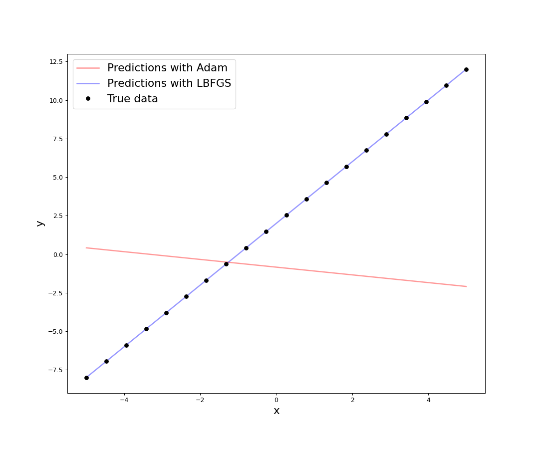
Woah! Look at that loss! LBFGS takes the loss almost to zero after just twenty epochs. Actually even before that, around five epochs. The loss seems to indicate that LBFGS is performing much better than Adam, but it is best to compare the performances by doing some predictions with the models trained with the different optimizers.
import matplotlib.pyplot as plt

x_for_pred = torch.linspace(-5, 5, steps=60).reshape(-1, 1).to(device)
with torch.no_grad():
    y_pred_adam = lm_adam(Variable(x_for_pred)).cpu().data.numpy()
    y_pred_lbfgs = lm_lbfgs(Variable(x_for_pred)).cpu().data.numpy()


# Training data
num_training_points = x.shape[0]
x_plot = x.reshape(num_training_points,).cpu().data.numpy()
y_plot = y.reshape(num_training_points,).cpu().data.numpy()

# Prediction data
num_pred_points = x_for_pred.shape[0]
x_for_pred = x_for_pred.reshape(num_pred_points,).cpu().data.numpy()
y_pred_adam = y_pred_adam.reshape(num_pred_points,)
y_pred_lbfgs = y_pred_lbfgs.reshape(num_pred_points,)

fig, ax = plt.subplots(figsize=(12, 10))
ax.plot(x_for_pred, y_pred_adam, "r", label="Predictions with Adam", alpha=0.4, lw=2)
ax.plot(x_for_pred, y_pred_lbfgs, "b", label="Predictions with LBFGS", alpha=0.4, lw=2)
ax.plot(x_plot, y_plot, "ko", label="True data")
ax.set_xlabel(r"x", fontsize="xx-large")
ax.set_ylabel(r"y", fontsize="xx-large")
ax.legend(fontsize="xx-large")
plt.savefig("linear_regression_with_Adam_LBFGS.png", dpi=90)
plt.close()

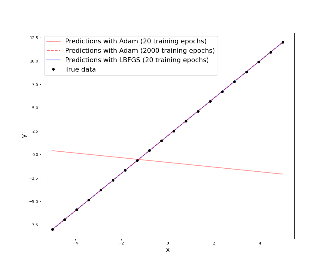
The graph shows what the loss hinted. For this simple model with a small synthetic dataset, LBFGS gives far superior performance than Adam. It is possible that with more training epochs, Adam will converge to a similar result.
lm_adam_2000 = LinearModel()
lm_adam_2000.to(device)
optimizer = Adam(lm_adam_2000.parameters(), weight_decay=0.0001)

epochs = 2000
for epoch in range(epochs):
    running_loss = 0.0

    for i, (x, y) in enumerate(dummy_data):

        x_ = Variable(x, requires_grad=True)
        y_ = Variable(y)

        # Forward pass
        y_pred = lm_adam_2000(x_)

        # Compute loss
        loss = criterion(y_pred, y_)

        # Zero gradients, backward pass, and update weights
        optimizer.zero_grad()
        loss.backward()
        optimizer.step()

        # Update the running loss
        running_loss += loss.item()

    if epoch % 100 == 0 or epoch == 1999:
        print(f"Epoch: {epoch + 1 if epoch == 0 or epoch == 1999 else epoch:04}/{epochs} Loss: {running_loss:.5e}")
Epoch: 0001/2000 Loss: 5.73596e+02
Epoch: 0100/2000 Loss: 7.65763e+01
Epoch: 0200/2000 Loss: 4.06436e+00
Epoch: 0300/2000 Loss: 2.67549e-02
Epoch: 0400/2000 Loss: 4.06526e-07
Epoch: 0500/2000 Loss: 2.26114e-07
Epoch: 0600/2000 Loss: 2.22508e-07
Epoch: 0700/2000 Loss: 2.34091e-07
Epoch: 0800/2000 Loss: 2.30016e-05
Epoch: 0900/2000 Loss: 4.25104e-04
Epoch: 1000/2000 Loss: 1.73270e-03
Epoch: 1100/2000 Loss: 3.28243e-03
Epoch: 1200/2000 Loss: 2.20446e-03
Epoch: 1300/2000 Loss: 2.36646e-03
Epoch: 1400/2000 Loss: 2.51782e-03
Epoch: 1500/2000 Loss: 2.40206e-03
Epoch: 1600/2000 Loss: 2.42837e-03
Epoch: 1700/2000 Loss: 2.44043e-03
Epoch: 1800/2000 Loss: 2.42643e-03
Epoch: 1900/2000 Loss: 2.43122e-03
Epoch: 2000/2000 Loss: 2.35328e-03
import matplotlib.pyplot as plt

x_for_pred = torch.linspace(-5, 5, steps=60).reshape(-1, 1).to(device)
with torch.no_grad():
    y_pred_adam = lm_adam(Variable(x_for_pred)).cpu().data.numpy()
    y_pred_adam_2000 = lm_adam_2000(Variable(x_for_pred)).cpu().data.numpy()
    y_pred_lbfgs = lm_lbfgs(Variable(x_for_pred)).cpu().data.numpy()


# Training data
num_training_points = x.shape[0]
x_plot = x.reshape(num_training_points,).cpu().data.numpy()
y_plot = y.reshape(num_training_points,).cpu().data.numpy()

# Prediction data
num_pred_points = x_for_pred.shape[0]
x_for_pred = x_for_pred.reshape(num_pred_points,).cpu().data.numpy()
y_pred_adam = y_pred_adam.reshape(num_pred_points,)
y_pred_adam_2000 = y_pred_adam_2000.reshape(num_pred_points,)
y_pred_lbfgs = y_pred_lbfgs.reshape(num_pred_points,)

fig, ax = plt.subplots(figsize=(12, 10))
ax.plot(x_for_pred, y_pred_adam, "r", label="Predictions with Adam (20 training epochs)", alpha=0.4, lw=2)
ax.plot(x_for_pred, y_pred_adam_2000, "r--", label="Predictions with Adam (2000 training epochs)", alpha=0.8, lw=2)
ax.plot(x_for_pred, y_pred_lbfgs, "b", label="Predictions with LBFGS (20 training epochs)", alpha=0.4, lw=2)
ax.plot(x_plot, y_plot, "ko", label="True data")
ax.set_xlabel(r"x", fontsize="xx-large")
ax.set_ylabel(r"y", fontsize="xx-large")
ax.legend(fontsize="xx-large")
plt.savefig("linear_regression_with_Adam_LBFGS_2000.png", dpi=90)
plt.close()

With a significantly larger number of training epochs (about 60 times), the performance of Adam comes close to that of LBFGS. It still remains to be seen if the third party implementations of the LBFGS optimizer gives a better performance than the builtin one, and how does LBFGS in general do when faced with nonlinear data, and/or deeper models. But for now LBFGS wins the crown.
Footnotes
The latest deep learning toolbox in Matlab includes a bunch of second
order optimizers - BFGS (trainbfg), Conjugate Gradient (traincgf,
traincgb, traincgp), Levenberg-Marquardt (trainlm, trainbr). I have not
seen any other machine learning library include so many second order optimizers.
Prior to this, I had only used the LBFGS optimizer that is implemented in SciPy, and that just worked. Scikit-learn actually uses this LBFGS optimizer.
Here are a couple of the third-party LBFGS optimizers for PyTorch:
- Stochastic LBFGS: http://sagecal.sourceforge.net/pytorch/index.html
- Modular LBFGS with weak Wolfe line search: https://github.com/hjmshi/PyTorch-LBFGS